Examples#
Henrik Boström, 2024
[1]:
import xrf
print(f"xrf v. {xrf.__version__}")
xrf v. 0.1.1
Classification forests#
Tic-tac-toe#
Let us start by importing the tic-tac-toe dataset from openml.org.
[2]:
from sklearn.datasets import fetch_openml
from sklearn.preprocessing import OneHotEncoder

dataset = fetch_openml(name="tic-tac-toe", parser="auto")

y = dataset.target.values

X_orig = dataset.data.values
X = OneHotEncoder().fit_transform(X_orig).toarray()
Let us split the dataset into a training and a test set.
[3]:
from sklearn.model_selection import train_test_split

X_train, X_test, y_train, y_test, X_orig_train, X_orig_test = train_test_split(
    X, y, X_orig, test_size=0.75)
Let us first generate a standard random forest classifier and apply it to the test set.
[4]:
from sklearn.ensemble import RandomForestClassifier
import numpy as np

np.random.seed(42)

rf = RandomForestClassifier(n_jobs=-1, n_estimators=500)
rf.fit(X_train, y_train)
rf_predictions = rf.predict_proba(X_test)
Similarly, we may generate and apply an explainable random forest classifier, here without constraining the number of training examples involved in the predictions.
[5]:
from xrf import XRandomForestClassifier

np.random.seed(42)

rfx = XRandomForestClassifier(n_jobs=-1, n_estimators=500)
rfx.fit(X_train, y_train)
rfx_predictions = rfx.predict_proba(X_test)
Let us check that we indeed get the same predictions.
[6]:
assert np.allclose(rf_predictions, rfx_predictions)
We may now limit the number of examples involved in a prediction, e.g., to at most 5 (k=5).
[7]:
k=5

rfx_predictions_k = rfx.predict_proba(X_test, k=k)
Let us compare the predictive performance of the original and the constrained predictions.
[8]:
from sklearn.metrics import roc_auc_score, accuracy_score
import pandas as pd

accuracy_orig = accuracy_score(y_test==rf.classes_[1],
                               np.round(rf_predictions[:,1]))
auc_orig = roc_auc_score(y_test == rf.classes_[1],
                         rf_predictions[:,1])

accuracy_k = accuracy_score(y_test==rfx.classes_[1],
                              np.round(rfx_predictions_k[:,1]))
auc_k = roc_auc_score(y_test == rfx.classes_[1],
                        rfx_predictions_k[:,1])

df_result = pd.DataFrame([[accuracy_orig, auc_orig],[accuracy_k, auc_k]],
                  index=["Original", f"k={k}"],
                  columns=["Accuracy", "AUC"])

display(df_result.round(3))
| Accuracy | AUC | |
|---|---|---|
| Original | 0.876 | 0.974 |
| k=5 | 0.933 | 0.982 |
Let us take a look at the example attribution for some prediction.
[9]:
rfx_predictions_k, examples, weights = rfx.predict_proba(
    X_test, k=k, return_examples=True, return_weights=True)
[10]:
rf_predicted_labels = np.array([rf.classes_[p.argmax()] for p in rf_predictions])
rfx_predicted_labels = np.array([rfx.classes_[p.argmax()] for p in rfx_predictions_k])
[11]:
def display_board(squares, Caption, Styles):
    df = pd.DataFrame(squares.reshape(3,3),
                      columns=["","",""],
                      index=["","",""])
    display(df.style.set_caption(Caption).set_table_styles(Styles))
[12]:
test_index = 0 # Select some test example

props = [("color", "grey"), ("font-weight", "bold")]
Styles = [dict(selector = "caption", props = props)]
props_b = [("caption-side", "bottom")]
Styles_b = [dict(selector = "caption", props = props_b)]

df = pd.DataFrame([rf_predictions[test_index]], index = [""],
                  columns=rf.classes_).round(2)
display(df.style.format(precision=2).set_caption("Original prediction").set_table_styles(Styles))

df = pd.DataFrame([rfx_predictions_k[test_index]], index = [""],
                  columns=rfx.classes_).round(2)
display(df.style.format(precision=2).set_caption("Constrained prediction").set_table_styles(Styles))

display_board(X_orig_test[test_index],
             f"Test example [{y_test[test_index]}]",
             Styles_b)

for i, e in enumerate(examples[test_index]):
    caption = f"Example #{i+1} [{y_train[e]}, {weights[test_index][i]:.2f}]"
    display_board(X_orig_train[examples[test_index][i]],
                 caption, Styles_b)
| negative | positive | |
|---|---|---|
| 0.37 | 0.63 |
| negative | positive | |
|---|---|---|
| 0.67 | 0.33 |
| x | o | x | |
| b | x | x | |
| o | o | o |
| b | b | x | |
| b | x | x | |
| o | o | o |
| b | o | x | |
| b | x | x | |
| o | o | x |
| x | b | x | |
| b | b | x | |
| o | o | o |
| x | x | b | |
| b | x | b | |
| o | o | o |
| x | o | o | |
| b | x | x | |
| o | b | x |
Let us check how many training examples contribute to the predictions in the original forest.
[13]:
import matplotlib.pyplot as plt

xrfc_predictions, all_non_zero_weights = rfx.predict_proba(X_test, c=1.0, return_weights=True)

lengths = [len(w) for w in all_non_zero_weights]

plt.hist(lengths, 10)
plt.xlabel("# training examples")
plt.ylabel("# test examples")
plt.show()

assert np.allclose(rf_predictions, xrfc_predictions)

Rather than constraining the predictions to a fixed number by setting a value for k, we could set a limit on the cumulative sum of the highest weights, e.g., to 30% (c=0.3).
[14]:
xrfc_predictions_c, all_non_zero_weights = rfx.predict_proba(
    X_test, c=0.3, return_weights=True)

lengths = [len(w) for w in all_non_zero_weights]

plt.hist(lengths, 10)
plt.xlabel("# training examples")
plt.ylabel("# test examples")
plt.show()

accuracy_c = accuracy_score(y_test==rfx.classes_[1],
                            np.round(xrfc_predictions_c[:,1]))
auc_c = roc_auc_score(y_test == rfx.classes_[1], xrfc_predictions_c[:,1])

df_result.loc["c=0.3"] = [accuracy_c, auc_c]
display(df_result.round(3))
| Accuracy | AUC | |
|---|---|---|
| Original | 0.876 | 0.974 |
| k=5 | 0.933 | 0.982 |
| c=0.3 | 0.932 | 0.985 |
MNIST#
Let us also consider the MNIST dataset at openml.org.
[15]:
dataset = fetch_openml(name="mnist_784", parser="auto")

X = dataset.data.values.astype(float)
y = dataset.target.values.astype(int)

print(f"Original dataset size: {X.shape}")
Original dataset size: (70000, 784)
Let us split the dataset into a training and a test set.
[16]:
from sklearn.model_selection import train_test_split

X_train, X_test, y_train, y_test, = train_test_split(
    X, y, test_size=0.1)
Let us first generate a standard random forest classifier and apply it to the test set.
[17]:
from sklearn.ensemble import RandomForestClassifier
import numpy as np

np.random.seed(42)

rf = RandomForestClassifier(n_jobs=-1, n_estimators=200)
rf.fit(X_train, y_train)
rf_predictions = rf.predict_proba(X_test)
Similarly, we may generate and apply an explainable random forest classifier, here without constraining the number of training examples involved in the predictions.
[18]:
from xrf import XRandomForestClassifier

np.random.seed(42)

rfx = XRandomForestClassifier(n_jobs=-1, n_estimators=200)
rfx.fit(X_train, y_train)
[18]:
XRandomForestClassifier(model=RandomForestClassifier(n_estimators=200, n_jobs=-1, oob_score=True)
[19]:
rfx_predictions, all_non_zero_weights = rfx.predict_proba(X_test, c=1.0, return_weights=True)
Let us check that we indeed get the same predictions.
[20]:
assert np.allclose(rf_predictions, rfx_predictions)
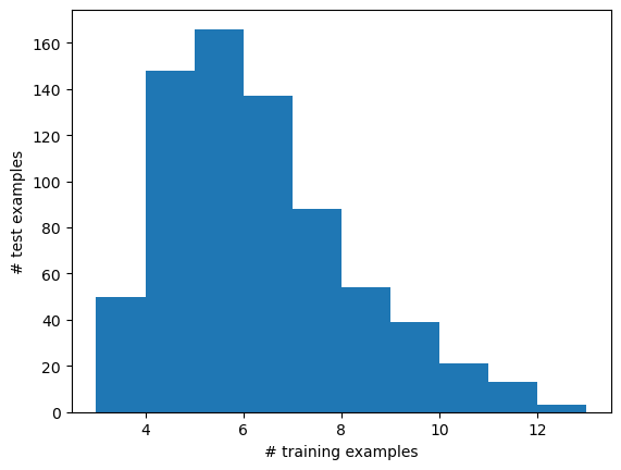
Let us check how many training examples contribute to the predictions.
[21]:
import matplotlib.pyplot as plt

lengths = [len(w) for w in all_non_zero_weights]

plt.hist(lengths, 10)
plt.xlabel("# training examples")
plt.ylabel("# test examples")
plt.show()

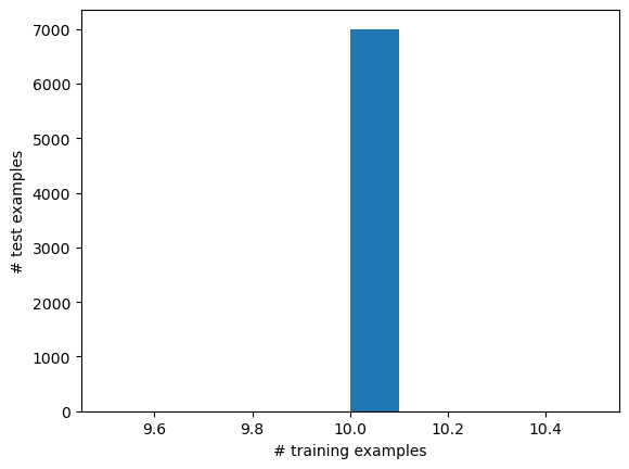
We may now limit the number of examples involved in a prediction, e.g., to at most 10 (k=10) and request that the top-weighted examples and the corresponding weights are returned.
[22]:
k=10

rfx_predictions_k, examples, weights  = rfx.predict_proba(X_test,
                                                          k=k,
                                                          return_examples=True,
                                                          return_weights=True)
[23]:
lengths = [len(w) for w in weights]

plt.hist(lengths, 10)
plt.xlabel("# training examples")
plt.ylabel("# test examples")
plt.show()
Let us compare the predictive performance of the original and the constrained predictions.
[24]:
rf_predicted_labels = np.array([rf.classes_[p.argmax()] for p in rf_predictions])
rfx_predicted_labels = np.array([rfx.classes_[p.argmax()] for p in rfx_predictions_k])
[25]:
from sklearn.metrics import roc_auc_score, accuracy_score

accuracy_orig = accuracy_score(y_test, rf_predicted_labels)
auc_orig = roc_auc_score(y_test, rf_predictions, average='weighted',
                         multi_class='ovr', labels=rf.classes_)

roc_auc_score(y_test == rf.classes_[1],
                         rf_predictions[:,1])

accuracy_k = accuracy_score(y_test, rfx_predicted_labels)
auc_k = roc_auc_score(y_test, rfx_predictions, average='weighted',
                      multi_class='ovr', labels=rfx.classes_)

df_result = pd.DataFrame([[accuracy_orig, auc_orig],[accuracy_k, auc_k]],
                  index=["Original", f"k={k}"],
                  columns=["Accuracy", "AUC"])

display(df_result.round(3))
| Accuracy | AUC | |
|---|---|---|
| Original | 0.965 | 0.999 |
| k=10 | 0.932 | 0.999 |
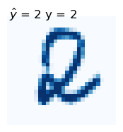
Let us take a look at the training examples that are used for some prediction.
[26]:
test_index = 5 # Select any test example
print("Test example:")
test_pixels = X_test[test_index].reshape((28, 28))
plt.figure(figsize=(2,2))
plt.imshow(test_pixels, cmap='Blues')
plt.axis('off')
plt.text(0.1, 0.1, r"$\hat{y}$" +f" = {rfx_predicted_labels[test_index]} y = {y_test[test_index]}",
fontsize = 12)
plt.show()
df = pd.DataFrame([rf_predictions[test_index]], index = [""], columns=rf.classes_)
display(df.style.format(precision=2).set_caption("Original prediction").set_table_styles(Styles))
df = pd.DataFrame([rfx_predictions_k[test_index]], index = [""], columns=rfx.classes_)
display(df.style.format(precision=2).set_caption("Constrained prediction").set_table_styles(Styles))
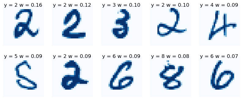
print("Training examples:")
no_rows = 2
no_cols = 5
fig, axs = plt.subplots(no_rows, no_cols, figsize=(10, 4))
for i, train_ind in enumerate(examples[test_index]):
pixels = X_train[train_ind].reshape((28, 28))
row = i // no_cols
col = i % no_cols
axs[row, col].imshow(pixels, cmap='Blues')
axs[row, col].axis('off')
axs[row, col].text(0.1, 0.5, f"y = {y_train[train_ind]} w = {weights[test_index][i]:.2f}", fontsize = 12)
plt.show()
Test example:
| 0 | 1 | 2 | 3 | 4 | 5 | 6 | 7 | 8 | 9 | |
|---|---|---|---|---|---|---|---|---|---|---|
| 0.03 | 0.01 | 0.58 | 0.03 | 0.08 | 0.03 | 0.17 | 0.01 | 0.06 | 0.01 |
| 0 | 1 | 2 | 3 | 4 | 5 | 6 | 7 | 8 | 9 | |
|---|---|---|---|---|---|---|---|---|---|---|
| 0.00 | 0.00 | 0.47 | 0.10 | 0.09 | 0.09 | 0.16 | 0.00 | 0.08 | 0.00 |
Training examples:
Regression forests#
Miami housing#
Let us import the Miami housing dataset from openml.org.
[27]:
from sklearn.datasets import fetch_openml
from sklearn.preprocessing import OneHotEncoder

dataset = fetch_openml(name="miami_housing", parser="auto")

y = dataset.target.values
X = dataset.data.values
Let us split the dataset into a training and a test set.
[28]:
from sklearn.model_selection import train_test_split

X_train, X_test, y_train, y_test = train_test_split(X, y, test_size=0.75)
Let us first generate a standard random forest regressor and apply it to the test set.
[29]:
from sklearn.ensemble import RandomForestRegressor
import numpy as np

np.random.seed(42)

rf = RandomForestRegressor(n_jobs=-1, n_estimators=500)
rf.fit(X_train, y_train)
rf_predictions = rf.predict(X_test)
Similarly, we may generate and apply an explainable random forest regressor, here without constraining the number of training examples involved in the predictions.
[30]:
from xrf import XRandomForestRegressor

np.random.seed(42)

rfx = XRandomForestRegressor(n_jobs=-1, n_estimators=500)
rfx.fit(X_train, y_train)
rfx_predictions = rfx.predict(X_test)
Let us check that we indeed get the same predictions.
[31]:
assert np.allclose(rf_predictions, rfx_predictions)
We may now limit the number of examples involved in a prediction, e.g., to at most 5 (k=5).
[32]:
k=5

rfx_predictions_k, examples, weights  = rfx.predict(X_test,
                                                    k=k,
                                                    return_examples=True,
                                                    return_weights=True)
Let us compare the correctness of the constrained and original predictions.
[33]:
from sklearn.metrics import mean_squared_error

rmse_orig = np.sqrt(mean_squared_error(y_test, rf_predictions))
corr_orig = np.corrcoef(y_test, rf_predictions)[0,1]

rmse_k = np.sqrt(mean_squared_error(y_test, rfx_predictions_k))
corr_k = np.corrcoef(y_test, rfx_predictions_k)[0,1]

df_result = pd.DataFrame([[rmse_orig, corr_orig],[rmse_k, corr_k]],
                  index=["Original", f"k={k}"],
                  columns=["RMSE", "CORR"])

display(df_result.round(3))
| RMSE | CORR | |
|---|---|---|
| Original | 111896.571 | 0.941 |
| k=5 | 113617.611 | 0.936 |
Let us take a look at the training examples that are used for some prediction.
[34]:
test_index = 0 # Select any test example
#test_index = np.argwhere(rfx_predicted_labels != y_test)[1,0] # Select a misclassified test example
#test_index = np.argwhere(rfx_predicted_labels != rf_predicted_labels)[2,0] # Select a test example on which there is disagreement

import pandas as pd

print(f"Original prediction: {rf_predictions[test_index]:.1f}")
print(f"Constrained prediction: {rfx_predictions_k[test_index]:.1f}")

df = pd.DataFrame(np.hstack((np.vstack((y_test[test_index], np.nan, X_test[test_index].reshape(-1,1))),
                             np.hstack((y_train[examples[test_index]].reshape(k,1),
                                        weights[test_index].reshape(k,1),
                                        X_train[examples[test_index]])).T)),
                            index = ["Target", "Weight"]+dataset.feature_names,
                  columns=["Test"]+["#"+str(i+1) for i in range(k)])

df.apply(pd.to_numeric).style.format(precision=2, thousands=" ", na_rep=" ").\
   background_gradient(cmap="Reds", axis=1)
Original prediction: 137202.8
Constrained prediction: 128643.4
[34]:
| Test | #1 | #2 | #3 | #4 | #5 | |
|---|---|---|---|---|---|---|
| Target | 133 000.00 | 168 000.00 | 115 000.00 | 115 000.00 | 120 000.00 | 81 500.00 |
| Weight | 0.33 | 0.20 | 0.19 | 0.15 | 0.14 | |
| LATITUDE | 25.89 | 25.90 | 25.89 | 25.89 | 25.88 | 25.86 |
| LONGITUDE | -80.23 | -80.23 | -80.24 | -80.23 | -80.23 | -80.23 |
| LND_SQFOOT | 7 575.00 | 8 925.00 | 7 200.00 | 8 100.00 | 5 300.00 | 8 025.00 |
| TOT_LVG_AREA | 1 176.00 | 1 251.00 | 1 170.00 | 884.00 | 1 264.00 | 1 178.00 |
| SPEC_FEAT_VAL | 1 512.00 | 1 176.00 | 3 088.00 | 0.00 | 0.00 | 2 197.00 |
| RAIL_DIST | 4 979.20 | 5 150.20 | 2 972.90 | 5 511.10 | 7 500.90 | 5 401.80 |
| OCEAN_DIST | 35 765.40 | 35 205.00 | 37 758.60 | 35 228.30 | 35 436.70 | 35 229.30 |
| WATER_DIST | 2 692.60 | 2 457.80 | 497.70 | 3 187.40 | 2 060.70 | 3 323.60 |
| CNTR_DIST | 43 454.60 | 44 715.80 | 43 128.10 | 43 460.00 | 37 986.10 | 30 764.50 |
| SUBCNTR_DI | 43 454.60 | 44 715.80 | 43 128.10 | 43 460.00 | 37 986.10 | 30 764.50 |
| HWY_DIST | 6 964.90 | 6 394.70 | 8 940.20 | 6 429.30 | 6 332.90 | 5 949.80 |
| age | 63.00 | 63.00 | 55.00 | 63.00 | 76.00 | 59.00 |
| avno60plus | 0.00 | 0.00 | 0.00 | 0.00 | 0.00 | 0.00 |
| month_sold | 3.00 | 2.00 | 1.00 | 10.00 | 3.00 | 3.00 |
| structure_quality | 4.00 | 4.00 | 4.00 | 4.00 | 4.00 | 4.00 |
Lipophilicty#
[35]:
import numpy as np
import pandas as pd
import rdkit
from rdkit.Chem import AllChem

url = ("https://deepchemdata.s3-us-west-1.amazonaws.com/datasets/"
       "Lipophilicity.csv")

df = pd.read_csv(url)

y = df["exp"].values

molecules = [rdkit.Chem.MolFromSmiles(s) for s in df["smiles"]]

fpgen = AllChem.GetMorganGenerator(radius=2, fpSize=1024)

X = np.array([fpgen.GetFingerprint(m) for m in molecules])

print(X.shape)
(4200, 1024)
Let us split the dataset into a training and a test set.
[36]:
from sklearn.model_selection import train_test_split

X_train, X_test, y_train, y_test, molecules_train, molecules_test = \
    train_test_split(X, y, molecules, test_size=0.75)
Let us first generate a standard random forest regressor and apply it to the test set.
[37]:
from sklearn.ensemble import RandomForestRegressor
import numpy as np

np.random.seed(42)

rf = RandomForestRegressor(n_estimators=500, n_jobs=-1)
rf.fit(X_train, y_train)
rf_predictions = rf.predict(X_test)
Similarly, we may generate and apply an explainable random forest regressor, here without constraining the number of training examples involved in the predictions.
[38]:
from xrf import XRandomForestRegressor

np.random.seed(42)

rfx = XRandomForestRegressor(n_estimators=500, n_jobs=-1)
rfx.fit(X_train, y_train)
rfx_predictions = rfx.predict(X_test)
Let us check that we indeed get the same predictions.
[39]:
assert np.allclose(rf_predictions, rfx_predictions)
We may now limit the number of examples involved in a prediction, e.g., to at most 10 (k=10).
[40]:
k=10

rfx_predictions_k, examples, weights  = rfx.predict(X_test,
                                                    k=k,
                                                    return_examples=True,
                                                    return_weights=True)
Let us compare the correctness of the constrained and original predictions.
[41]:
from sklearn.metrics import mean_squared_error

rmse_orig = np.sqrt(mean_squared_error(y_test, rf_predictions))
corr_orig = np.corrcoef(y_test, rf_predictions)[0,1]

rmse_k = np.sqrt(mean_squared_error(y_test, rfx_predictions_k))
corr_k = np.corrcoef(y_test, rfx_predictions_k)[0,1]

df_result = pd.DataFrame([[rmse_orig, corr_orig],[rmse_k, corr_k]],
                  index=["Original", f"k={k}"],
                  columns=["RMSE", "CORR"])

display(df_result.round(3))
| RMSE | CORR | |
|---|---|---|
| Original | 0.969 | 0.602 |
| k=10 | 1.013 | 0.567 |
Let us take a look at some test example and the training examples that are used for the prediction.
[42]:
import matplotlib.pyplot as plt

from rdkit import Chem
from rdkit.Chem.Draw import IPythonConsole
from rdkit.Chem import Draw
from rdkit.Chem import rdFMCS
from rdkit.Chem.Draw import rdDepictor

IPythonConsole.ipython_useSVG=False
IPythonConsole.drawOptions.minFontSize=20

rdDepictor.SetPreferCoordGen(True)

def show_difference(mol1, w, y, mol2):
    mcs = rdFMCS.FindMCS([mol1,mol2])
    mcs_mol = Chem.MolFromSmarts(mcs.smartsString)
    match1 = mol1.GetSubstructMatch(mcs_mol)
    target_atm1 = []
    for atom in mol1.GetAtoms():
        if atom.GetIdx() not in match1:
            target_atm1.append(atom.GetIdx())
    return Draw.MolsToGridImage([mol1],
                                highlightAtomLists=[target_atm1],
                                useSVG=True)
[43]:
test_index = 5 # Select any test example

print("Test molecule:")
test_mol = molecules_test[test_index]
test_mol_fig = Draw.MolsToGridImage([test_mol], useSVG=True)
display(test_mol_fig)
print(f"True target: {y_test[test_index]:.2f}")
print(f"Original prediction: {rf_predictions[test_index]:.2f}")
print(f"Constrained prediction: {rfx_predictions_k[test_index]:.2f}\n")

for i, training_index in enumerate(examples[test_index]):
    print(f"Training example {i+1} "
          f"[{y_train[training_index]}, "
          f"weight: {weights[test_index][i]:.2f}]")
    training_mol = molecules_train[training_index]
    train_mol_fig = show_difference(training_mol, weights[test_index][i],
                                    y_train[training_index], test_mol)
    display(train_mol_fig)
Test molecule:

True target: 1.42
Original prediction: 2.28
Constrained prediction: 2.58

Training example 1 [2.5, weight: 0.22]

Training example 2 [3.77, weight: 0.19]

Training example 3 [2.7, weight: 0.11]

Training example 4 [1.85, weight: 0.08]

Training example 5 [2.8, weight: 0.08]

Training example 6 [2.39, weight: 0.07]

Training example 7 [3.4, weight: 0.07]

Training example 8 [1.4, weight: 0.06]

Training example 9 [1.09, weight: 0.05]

Training example 10 [1.3, weight: 0.05]
